Variational inference in 5 minutes

Variational inference has a reputation of being really complicated or involving mathematical black magic. I think part of this is because the standard derivation uses Jensen’s inequality in a way that seems unintuitive. Here’s an derivation that feels easier to me, using only the notion of KL divergence between probability distributions.

Let $p(x,z)$ be a probability model with observed variables $x$ and latent variables $z$.¹ We want to infer the posterior $p(z|x)$, but in general this won’t have any nice form that we can write down. Instead, we’ll pick some approximating family $q(z;\lambda)$, with parameters $\lambda$, and then try to find the distribution within this family that best approximates the posterior. For example, if we model each latent variable independently (a “mean field” approximation) using a scalar Gaussian, the parameters $\lambda$ are just the means and standard deviations of these Gaussians.

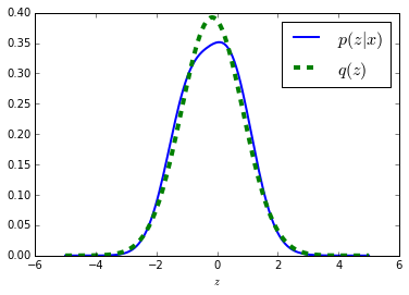
A variational Gaussian approximation to a scalar posterior.

A natural approach to fitting the approximation parameters $\lambda$ is to minimize the KL divergence between our approximation $q(z;\lambda)$ and the posterior $p(z|x)$.² Writing this out,

\begin{align} KL\left[q(z;\lambda) \| p(z|x)\right] &= \int q(z;\lambda) \log \frac{q(z;\lambda)}{p(z|x)} dz,\end{align}

we see that it depends on the posterior density $p(z|x)$ which we don’t know. However, we do have access to the joint distribution $p(x, z)$, which is proportional to the posterior, so we can just apply simple algebra to unpack the normalizing constant:

\begin{align} KL\left[q(z;\lambda) \| p(z|x)\right] &= \int q(z;\lambda) \log \frac{q(z;\lambda)}{p(z|x)} dz\\&= \int q(z;\lambda) \left[\log q(z;\lambda) - \log p(z|x)\right] dz\\&= \int q(z;\lambda) \left[\log q(z;\lambda) - \log \frac{p(x,z)}{p(x)}\right] dz\\&= \log p(x) + \int q(z;\lambda) \left[\log q(z;\lambda) - \log p(x,z) \right] dz\\&= \log p(x) - \mathcal{F}(\lambda; x).\end{align}

This shows that the KL divergence is equal to the model evidence $\log p(x)$, which is an (unknown) normalizing constant, minus a term $\mathcal{F}$ given by \[\mathcal{F}(\lambda; x) = \int q(z;\lambda) \left[ \log p(x,z) - \log q(z;\lambda)\right] dz.\] This term is alternately referred to as (negative) variational free energy or the evidence lower bound (ELBO). It is a lower bound on $\log p(x)$ because we can write $\log p(x) = \mathcal{F} + KL\left[q(z;\lambda)\|p(z|x)\right]$ and the KL divergence is nonnegative. Since the model evidence is constant, maximizing $\mathcal{F}$ minimizes the KL divergence.

This is the core of variational inference: pick an approximating family and minimize KL divergence between your approximation and the true posterior. If you just do this, you will naturally derive the variational bound $\mathcal{F}$ without any algebraic tricks or appeals to Jensen’s inequality.

The practical difficulty tends to be that $\mathcal{F}$ involves an expectation, so evaluating and optimizing it requires either model-specific math³ or Monte Carlo techniques. In the next post I’ll describe the simple Monte Carlo method used by Stan (among others) to perform variational inference in any model where gradients are available.